


Table of Contents
- Four Families, Not One Ranking
- Classical: ARIMA and ETS
- Prophet and NeuralProphet
- Gradient Boosting: XGBoost and LightGBM
- Deep Learning: N-BEATS, TFT, PatchTST
- Foundation Models: TimeGPT, Chronos, TimesFM
- Head to Head
- How to Choose in Five Minutes
- A Worked Decision on One Dataset
- When Forecasts Have to Add Up
- The Part Everyone Gets Wrong
- Seven Mistakes That Ruin Forecasts
- What Each Approach Costs to Run
- Frequently Asked Questions
- Final Thoughts
Ask which forecasting model is best and you will get an answer that depends entirely on who you asked. The statistician says ARIMA. The Kaggle competitor says gradient boosting. The person who read a paper last week says foundation models.
They are all partly right, because forecasting models because these approaches are not competing on one axis. They differ in what they assume about your data, how much of it they need, and whether anyone has to be able to explain the output.

Forecasting Models Split Into Four Families
The field in 2026 splits cleanly into four groups.
Classical statistical methods — ARIMA, SARIMAX, ETS. Decades old, mathematically well understood, still the right answer more often than people expect.
Additive decomposition models — Prophet and its descendants. Designed for business series with holidays, trends and seasonality.
Gradient boosting on engineered features. XGBoost, LightGBM. Not forecasting models by design; extremely effective when you frame forecasting as a supervised problem.
Deep learning and foundation models. N-BEATS, TFT, PatchTST, and the newer zero-shot models like TimeGPT, Chronos and TimesFM.
Despite all the attention on the last group, classical and task-specific methods like SARIMAX, Prophet and gradient boosting remain the most widely used in operational forecasting, particularly where interpretability and low data requirements matter more than the last few points of accuracy.
Classical: ARIMA and ETS
ARIMA models a series as a function of its own past values and past errors. ETS decomposes it into error, trend and seasonal components.
What they are genuinely good at. Short series. A few dozen observations is enough, where machine learning approaches need hundreds. They produce well-calibrated prediction intervals rather than point estimates, which matters more than accuracy in most business contexts. And you can explain exactly why the forecast is what it is.
Where they struggle. Multiple seasonalities, external variables beyond what SARIMAX handles, and long horizons. They also require the series to be reasonably stationary after differencing, which takes judgement.
Use them when: you have one series, limited history, and someone will ask you to justify the number. This describes a surprising amount of real forecasting work.
Prophet and NeuralProphet
Prophet is an additive regression model built for business and operational series, trend, seasonality and holiday effects, fitted with sensible defaults.
Its real contribution was accessibility. Analysts who would never tune an ARIMA model could produce a reasonable forecast with holiday effects in ten lines. That democratisation was genuinely valuable.
The honest assessment. Benchmarks consistently show Prophet with higher errors than both classical methods and gradient boosting on many datasets, and notably slow prediction times. It is not the accuracy leader and was never designed to be.
Where it still wins. Explainability. You can show a stakeholder the trend component, the weekly seasonality and the holiday effects as separate charts. When the forecast must be understood rather than merely accurate, that decomposition is worth real accuracy.
NeuralProphet keeps the interpretable structure and adds autoregression, which helps considerably when the data has strong short-term patterns Prophet’s smooth trend misses.
Gradient Boosting: XGBoost and LightGBM
The pragmatist’s answer, and frequently the one that wins.
Using LightGBM or similar, you reframe forecasting as supervised learning: build features from lags, rolling statistics, calendar effects and external variables, then predict the target. The model has no concept of time. You encode it in the features.
Why it works so well. Handles many external variables naturally. Learns nonlinear interactions. Trains fast. And it scales across thousands of series in one model, which is how most retail and demand forecasting actually operates.
Benchmark comparisons consistently place LightGBM among the strongest accuracy-per-unit-of-compute options available.
The catch. Feature engineering is the whole job, and it is where the skill lives. It also extrapolates badly, a tree cannot predict a value outside its training range, which makes trending series a genuine problem unless you model the trend separately or predict differences.
Deep Learning: N-BEATS, TFT, PatchTST
Purpose-built neural architectures for sequences.
N-BEATS uses stacked residual blocks and performs strongly on standard benchmarks. Temporal Fusion Transformer handles multiple series with static and time-varying covariates, and provides attention-based interpretability. PatchTST applies transformer patching to time series with strong results on long horizons.
The trade. Benchmarks show neural approaches achieving the lowest errors on suitable data, and taking by far the longest to train. They also need substantial history. Below a few thousand observations they typically lose to simpler methods.
Use them when: you have many long series, accuracy justifies the engineering, and you have someone who can debug a training run.
Foundation Models: TimeGPT, Chronos, TimesFM
The genuinely new development, and the one worth understanding properly.
These are large models pre-trained on enormous collections of time series, which then forecast your series without being trained on it. Zero-shot forecasting.
TimeGPT works through a managed API, send your series, receive a forecast, no infrastructure. Chronos (AWS) takes the open-weight route, tokenising time series values so a language-model architecture can handle them. TimesFM (Google) is similarly open and pre-trained.
Both Chronos and TimesFM deliver competitive zero-shot performance on the Monash forecasting benchmarks without any fine-tuning, which is a genuinely surprising result, a model that never saw your data performing comparably to one trained on it.
Where they fit. Fast results without training infrastructure. Cold-start problems where you have almost no history. Probabilistic forecasts, which they handle well. And situations where you have thousands of series and cannot maintain a model per series.
The caution. They are harder to explain, you inherit whatever biases the pre-training data carried, and the managed options mean sending your data to an API. Benchmark performance on public datasets does not guarantee performance on your particular series, test before committing.
Head to Head
| Approach | Data needed | Training speed | Explainability | Best for |
|---|---|---|---|---|
| ARIMA / ETS | Very low | Fast | High | Single series, short history |
| Prophet | Low | Moderate | Very high | Business series needing explanation |
| NeuralProphet | Moderate | Moderate | High | Strong short-term patterns |
| LightGBM / XGBoost | Moderate | Fast | Moderate | Many covariates, many series |
| N-BEATS / TFT / PatchTST | High | Slow | Low to moderate | Long horizons, large datasets |
| TimeGPT / Chronos / TimesFM | Very low (zero-shot) | None required | Low | Cold start, many series, speed |
How to Choose Forecasting Models in Five Minutes
- Under a hundred observations? ARIMA or ETS. Nothing else has enough to learn from.
- Does someone need the forecast explained? Prophet, for the decomposition alone.
- Do you have useful external variables? Gradient boosting. Nothing else absorbs covariates as easily.
- Thousands of series with no time to model each? A foundation model, or one gradient boosting model across all of them.
- Long history, long horizon, accuracy is the whole point? Deep learning, and budget the engineering time.
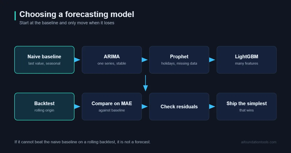
- Genuinely unsure? Run a seasonal naive baseline, then ARIMA, then LightGBM. If neither beats the baseline meaningfully, the problem is your data.
That last point matters more than the rest. A seasonal naive forecast, this week equals the same week last year, beats sophisticated forecasting models more often than anyone admits publicly.
A Worked Decision on One Dataset
Concrete beats abstract. Say you forecast weekly demand for eight hundred retail products, three years of history, with promotions and price changes recorded.
Seasonal naive first. This week equals the same week last year. Takes ten minutes and establishes whether the problem is even hard. Frequently it is embarrassingly competitive.
ARIMA per product is the wrong shape here. Eight hundred models to fit, tune and maintain, none of which can use promotion data. Classical forecasting models excel on one series with limited history, and this is neither.
Prophet per product has the same problem plus slower prediction. Its strength – explaining a single series to a stakeholder – is not what you need across eight hundred SKUs.
Gradient boosting across all products is the natural fit. One model, product identity as a feature, promotions and prices as covariates, lags and rolling means engineered from history. It learns patterns shared across products, which is exactly the structure retail data has.
A foundation model is worth benchmarking for the new products with no history, where every other approach has nothing to work with. This cold-start case is where zero-shot genuinely earns its place.
Note that the decision was driven entirely by the shape of the problem – many related series, useful covariates, some cold starts – and not at all by which method is most accurate in the abstract.
When Forecasts Have to Add Up
A constraint that catches people out, and it has nothing to do with model choice.
If you forecast by product, by region and in total, those numbers need to be consistent. Forecast each level independently and they will not reconcile – the sum of your regional forecasts will differ from your national one, and someone will notice in a board meeting.
Two approaches. Bottom-up forecasts the lowest level and sums upward, which is simple and inherits noise from sparse series. Reconciliation methods forecast every level independently then adjust them to be coherent, usually with better accuracy at the top.
This matters because hierarchical structure is extremely common in business forecasting and almost absent from tutorials. If your forecasts feed a planning process with multiple levels, reconciliation is not optional regardless of which forecasting models you chose.
The Part Everyone Gets Wrong
Validation, and it invalidates more forecasting work than any modelling choice.
Never use a random train-test split. Time series data is ordered. Randomly holding out points means training on the future to predict the past, which produces spectacular results that collapse in production.
Use rolling-origin backtesting. Hyndman and Athanasopoulos cover the method properly. Train up to a point, forecast forward, step the origin, repeat. This mirrors how the model will actually be used and gives you error at each horizon rather than one aggregate number.
Match your test horizon to your real one. If you forecast fourteen days ahead in production, evaluate at fourteen days. Accuracy degrades with horizon, and one-step-ahead error tells you almost nothing about day fourteen.
Always compare against naive baselines. Seasonal naive and drift. A model that does not beat both is not a model, whatever its error metric says.
Get this wrong and every comparison in this article becomes meaningless for your case.
Seven Mistakes That Ruin Forecasts
1. Leaking future information. Using a feature not available at prediction time. The most common and most damaging error.
2. Forecasting the wrong thing. Often the useful quantity is a difference or a rate, not a level.
3. Ignoring prediction intervals. A point forecast without uncertainty is a guess presented as a fact. Business decisions need the range.
4. Optimising the wrong metric. MAPE breaks near zero and punishes over-forecasting asymmetrically. Choose a metric that reflects the actual cost of being wrong.
5. Retraining without monitoring. Scheduled retraining on drifted data can make forecasts worse. Our guide to MLOps covers the monitoring side.
6. Treating outliers as signal. One pandemic, one outage, one promotion. Handle them explicitly or they distort everything.
7. No human review. Forecasters who never look at the chart miss obvious failures a glance would catch.
What Each Approach Costs to Run
Accuracy comparisons dominate the discussion. Operating cost decides what survives contact with production.
Classical methods are nearly free. Fitting ARIMA on a few hundred points is milliseconds. The cost is human – someone has to check stationarity and choose orders, and that judgement does not automate cleanly across many series.
Gradient boosting is cheap to train, expensive to maintain. The model trains in seconds. The feature pipeline behind it is real engineering, and it has to run identically at training and prediction time or your forecasts quietly degrade.
Deep learning is expensive on both axes. Training runs measured in hours, hyperparameters to tune, and a debugging burden when something stops converging. Justifiable when accuracy translates directly into money.
Foundation models invert the pattern. No training cost at all, but per-call API cost on the managed options, or the hardware to run the open ones. For a handful of series this is trivial; across thousands of daily forecasts it becomes a real line item worth modelling before you commit.
The pattern worth noticing: forecasting models that look cheapest in a benchmark often cost most in production, because benchmarks measure training and production is mostly maintenance.
Frequently Asked Questions
Is Prophet still worth using?
For explainability, yes. For pure accuracy, gradient boosting or classical methods frequently beat it. Choose it when the decomposition into trend, seasonality and holidays is what stakeholders need to see.
Do foundation models replace traditional forecasting?
Not yet, and possibly not for many use cases. They are excellent for cold start and scale, weaker on explainability, and their benchmark performance does not automatically transfer to your data.
How much history do I need?
Two full seasonal cycles at minimum for anything seasonal. More is better for machine learning approaches; foundation models relax this considerably.
What metric should I use?
MAE for interpretability, RMSE when large errors are disproportionately costly, and a scaled metric like MASE when comparing across series of different magnitudes. Avoid MAPE on data near zero.
Can I forecast with an LLM?
General language models are poor at numerical forecasting. Purpose-built time series foundation models are a different thing and genuinely capable, do not confuse the two.
Should I build one model per series or one across all?
One global model across many series usually wins when the series are related, because it learns shared patterns. Individual models win when series behave very differently.
Final Thoughts
The pattern across every honest benchmark is that no family dominates. Classical methods win on short series, gradient boosting wins when covariates matter, deep learning wins with enough data and patience, and foundation models win on speed and cold start.
What consistently separates good forecasting work from bad is not the model. It is proper backtesting, a naive baseline, honest prediction intervals and a metric that reflects the real cost of error.
Start with seasonal naive. Add ARIMA. Try LightGBM with sensible features. If none of them beat the baseline convincingly, more sophisticated forecasting models will not rescue you, the signal is not there, and knowing that is a genuinely useful result.